Required Practical: Inverse Square-Law for Gamma Radiation
Aim of the Experiment
The aim of this experiment is to verify the inverse square law for gamma radiation of a known gamma-emitting source
Variables
- Independent variable = the distance between the source and detector, x (m)
- Dependent variable = the count rate / activity of the source, C
- Control variables
- The time interval of each measurement
- The same thickness of aluminium foil
- The same gamma source
Equipment List

- Resolution of equipment:
- Metre ruler = 1 mm
- Stopwatch = 0.01 s
Method

Set up for inverse-square law investigation
- Measure the background radiation using a Geiger Muller tube without the gamma source in the room, take several readings and find an average
- Next, put the gamma source at a set starting distance (e.g. 5 cm) from the GM tube and measure the number of counts in 60 seconds
- Record 3 measurements for each distance and take an average
- Repeat this for several distances going up in 5 cm intervals
- A suitable table of results might look like this:

Analysing the Results
- According to the inverse square law, the intensity, I, of the γ radiation from a point source depends on the distance, x, from the source

- Intensity is proportional to the corrected count rate, C, so

- Comparing this to the equation of a straight line, y = mx
- y = C (counts min–1)
- x = 1/x2 (m–2)
- Gradient = constant, k
- Square each of the distances and subtract the background radiation from each count rate reading
- Plot a graph of the corrected count rate per minute against 1/x2
- If it is a straight line graph through the origin, this shows they are directly proportional, and the inverse square relationship is confirmed

A straight-line graph verifies the inverse square relationship. The closer the points are to the line, the better the experiment has demonstrated the relationship
Evaluating the Experiment
Systematic errors:
- The Geiger counter may suffer from an issue called “dead time”
- This is when multiple counts happen simultaneously within ~100 μs and the counter only registers one
- This is a more common problem in older detectors, so using a more modern Geiger counter should reduce this problem
- The source may not be a pure gamma emitter
- To prevent any alpha or beta radiation being measured, the Geiger-Muller tube should be shielded with a sheet of 2–3 mm aluminium
Random errors:
- Radioactive decay is random, so repeat readings are vital in this experiment
- Measure the count over the longest time span possible
- A larger count helps reduce the statistical percentage uncertainty inherent in smaller readings
- This is because the percentage error is proportional to the inverse-square root of the count
Safety Considerations
- For the gamma source:
- Reduce the exposure time by keeping it in a lead-lined box when not in use
- Handle with long tongs
- Do not point the source at anyone and keep a large distance (as activity reduces by an inverse square law)
- Safety clothing such as a lab coat, gloves and goggles must be worn
Worked example
A student measures the background radiation count in a laboratory and obtains the following readings: The student is trying to verify the inverse square law of gamma radiation on a sample of Radium-226. He collects the following data:
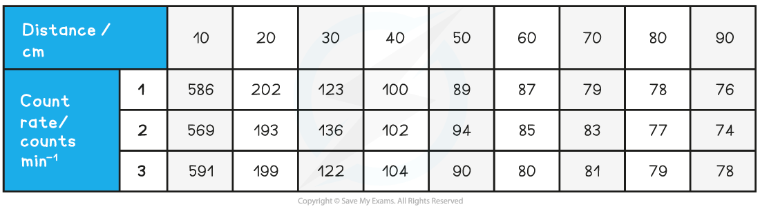 Use this data to determine if the student’s data follows an inverse square law. Determine the uncertainty in the gradient of the graph.
Step 1: Determine a mean value of background radiation

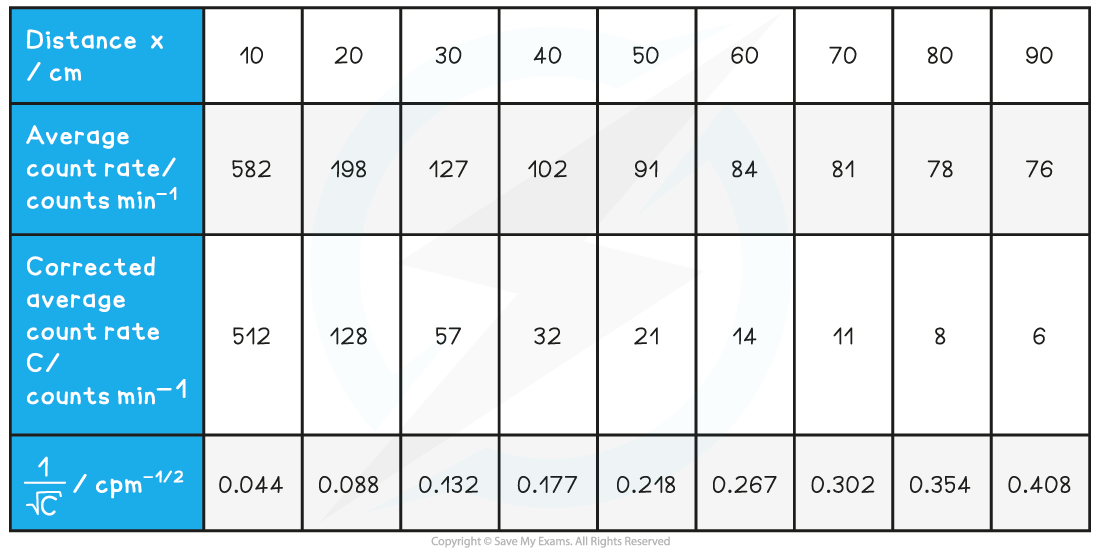
Step 2: Calculate C (corrected average count rate) and C–1/2
Step 3: Plot a graph of C–1/2 against x and draw a line of best fit
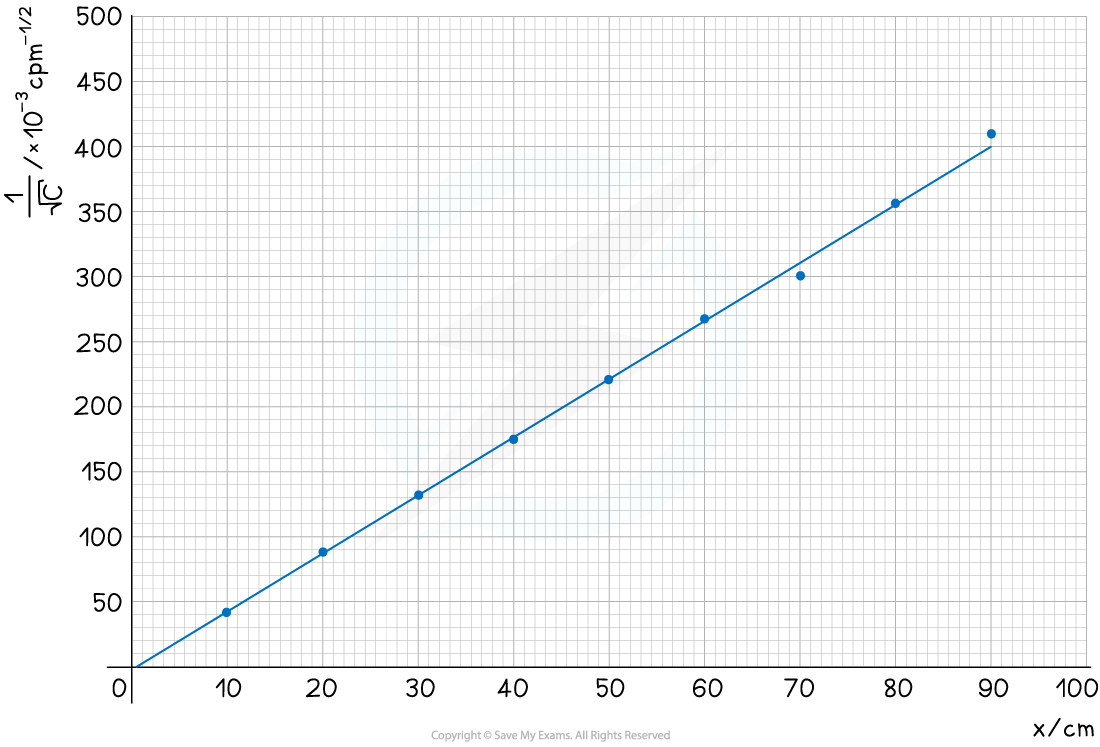
- The graph shows C–1/2 is directly proportional to x, therefore, the data follows an inverse square law
Step 4: Determine the uncertainties in the readings


Step 5: Plot the error bars and draw a line of worst fit

Step 6: Calculate the uncertainty in the gradient